Deep Dive into Word Cloud Creation

Introduction
Motivation
While working on the F1 Trending Tweets dataset, I saw an opportunity to take a deeper dive into optimizing word clouds. I found that creating clear and informative word clouds required some careful tuning and customization. This process inspired me to share the insights I gained, in the hope that they can help others improve their own word cloud visualizations.
The goal of this post is to provide practical tips and techniques for crafting more effective word clouds. By addressing common issues like redundant words, color choices, and shape customization, I aim to help you create word cloud visualizations that truly enhance your data analysis workflow. You won’t have to struggle with subpar word clouds anymore — instead, you can focus your efforts on other important steps in the data analysis process.
Data Overview
This project is based on a dataset of trending tweets related to Formula 1 (F1). The dataset contains the following key information:
- Text: The content of the tweets.
- User Information: Details like user location, follower count, and verified status.
- Hashtags: Tweets containing the #F1 hashtag and related trending keywords.
- Date: Tweets posted from March 2022 to July 2022, covering the first half of the 2022 racing season.
I used the text data from these tweets as the foundation for generating word clouds. I focused on cleaning the text, handling stopwords, and using a custom colormap. This would make the visualizations more impactful.
User Location Distribution After Mapping

As part of the exploratory data analysis (EDA) process, I visualized the distribution of user locations using a bar chart. As expected, given Formula 1’s strong British heritage, the UK had the highest number of tweets, except for “Worldwide” which was the top category.
The high volume of UK tweets shows a strong interest in F1 content about the British GP, UK teams, and drivers from the UK. It highlights this region's strong interest and influence within the F1 community.
This analysis of the user location data provides important context for understanding the word cloud insights that will be presented later in the post. The prominence of the UK in the F1 conversation helps explain some of the patterns we may observe in the textual analysis.
Word Cloud Creation Process

Before delving into the details of my F1 tweet word cloud analysis, let’s briefly discuss what word clouds are and their purpose.
Word clouds are a visual representation of text data. The size and prominence of words reflect their frequency. The example above shows a Korean word cloud. I made it in a previous project using the ‘wordcloud’ library in R.
Word clouds can be a useful tool in text analysis, as they help summarize key themes and enhance the visual appeal of textual data. One of the most convenient aspects of word clouds is the ease of creating them, thanks to the ‘wordcloud’ libraries available in Python and R, as well as various online tools.
For the F1 tweet analysis, I used these word cloud creation capabilities to gain insights into the most prominent terms and topics discussed within the dataset. However, as I soon discovered, achieving truly effective and informative word clouds required some additional customization and fine-tuning.
In the following sections, I’ll share the specific steps I took to enhance the clarity and impact of my F1 tweet word clouds. These learnings can help you create more impactful word cloud visualizations for your text-based datasets.
Topics Covered:
- Basic Word Cloud Creation
- Advanced Customizations
- Visualization and Aesthetics
Basic Word Cloud Creation
Using the ‘wordcloud’ Library:
Installation: Ensure you have the necessary libraries installed. You can install them using pip if they’re not already available:
pip install wordcloud matplotlib numpy pillowImporting Libraries: Import the required libraries for creating and visualizing word clouds:
from wordcloud import WordCloud, STOPWORDS
import matplotlib.pyplot as plt
import numpy as np
from PIL import Image
from matplotlib.colors import LinearSegmentedColormap
import re
Basic Parameters: When creating a word cloud, you can customize several parameters to control its appearance:
widthandheight: Define the dimensions of the word cloud.background_color: Sets the background color of the word cloud.max_words: Limits the maximum number of words displayed.
Generating a Simple Word Cloud: Here’s a basic example of generating a word cloud using the default settings:
# Define your text data
text = "Your sample text data goes here."

# Generate a basic word cloud
wordcloud = WordCloud(
    width=800,  # Set the width of the word cloud
    height=400,  # Set the height of the word cloud
    background_color='white'  # Set the background color
).generate(text)

# Display the word cloud
plt.figure(figsize=(10, 5))  # Adjust the figure size
plt.imshow(wordcloud, interpolation='bilinear')  # Smooth rendering
plt.axis('off')  # Hide the axis
plt.title('Basic Word Cloud')  # Add a title
plt.show()  # Render the plot
Explanation:
WordCloudConstructor: Creates aWordCloudobject with specified dimensions and background color.generate(text): Processes the text to generate the word cloud.imshow(): Renders the word cloud image.axis('off'): Hides the axis for a cleaner look.show(): Displays the word cloud.
Advanced Customizations
Let’s dive into the advanced customizations I applied to create more impactful word clouds for the F1 Trending Tweets dataset.
Stopwords and Filtering:
- Defining Stopwords: Customizing the list of stopwords is essential for filtering out common or irrelevant words from the word cloud. This ensures the most significant terms are highlighted. In this case, I included the term “F1” among the stopwords to refine the output. Despite attempts to normalize all variations of “F1” using
re.sub, I ultimately chose to remove the term entirely since all tweets already included the F1 hashtag. This approach helps to better emphasize other key terms. - Preprocessing Text: Cleaning and preparing the text data is crucial for generating accurate visualizations. This step involves normalizing variations of keywords, such as standardizing “F1” to a consistent format, and removing unwanted characters or noise from the text. Proper preprocessing ensures the final word cloud effectively represents the key themes and terms.
Here’s the code that demonstrates these steps:
# Define custom stopwords
custom_stopwords = set(STOPWORDS).union({
'RT', 'https', 'the', 'and', 'of', 'to', 'will', 'much', 'see', 'now', 'seen',
'come', 'know', 'haa', 'football club', 'even', 't', 'co', 'f1oki f1okidao',
'far', 'take', 'don', 'f1okidao', 'f1okidao doge', 'thing',
'got', 'really', 's', 'u', 'still', 'way', 'f1'
})
# Combine all text data into a single string without changing case
all_text = ' '.join(f1['text'].fillna(''))
# Remove unnecessary variations and normalize terms like "F1"
all_text = re.sub(r'\bf1\b', 'F1', all_text, flags=re.IGNORECASE) # Replace "f1" with "F1"
all_text = re.sub(r'#f1\b', 'F1', all_text, flags=re.IGNORECASE) # Replace #f1 with F1
all_text = re.sub(r'\bf1gp\b', 'F1', all_text, flags=re.IGNORECASE) # Replace f1gp with F1
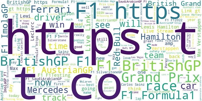
# Generate the word cloud using the custom stopwords and colormap
wordcloud = WordCloud(
width=800,
height=400,
stopwords=custom_stopwords, # Apply custom stopwords
background_color='white', # White background for contrast
colormap='viridis' # Custom colormap
).generate(all_text)
# Display the word cloud
plt.figure(figsize=(10, 6)) # Adjust the figure size for better display
plt.imshow(wordcloud, interpolation='bilinear') # Smooth rendering
plt.axis('off') # Hide the axis
plt.title('Word Cloud of F1 Tweets with Custom Stopwords') # Add a title
plt.show() # Render the plot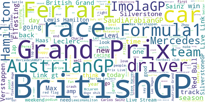
Colormaps and Custom Colors:
Next, let’s explore how you can use predefined and custom colormaps to enhance the visual appeal of your word clouds.
- Predefined Colormaps: Matplotlib provides a wide range of built-in colormaps to apply to your word clouds. These predefined colormaps offer diverse color schemes, allowing you to experiment and find the most suitable palette for your data. Some popular options include
colormap='viridis'for a vibrant, multi-color gradient,colormap='plasma'for a warm color palette, andcolormap='cividis'for a colorblind-friendly option. You can easily adjust these colormaps to match the theme or aesthetic of your project. - Custom Colormaps: For a more personalized touch, you can create and apply custom colormaps tailored to specific themes. For instance, you might use colors inspired by F1 teams for a themed word cloud.
Here’s how you can create and apply a custom colormap:
# Define a custom colormap inspired by F1 team-related colors
f1_theme_cmap = LinearSegmentedColormap.from_list('f1_theme', ['#00D2BE', '#000000', '#C0C0C0'])

# Generate the word cloud using the custom colormap and stopwords
wordcloud = WordCloud(
    width=800,
    height=400,
    stopwords=custom_stopwords,  # Apply custom stopwords
    background_color='white',  # White background for contrast
    colormap=f1_theme_cmap  # Use the custom colormap
).generate(all_text)

# Display the word cloud
plt.figure(figsize=(10, 5))  # Adjust figure size for better display
plt.imshow(wordcloud, interpolation='bilinear')  # Smooth rendering
plt.axis('off')  # Hide the axis
plt.title('Word Cloud of F1 Tweets with Custom Colormap and Stopwords')  # Add a title
plt.show()  # Render the plot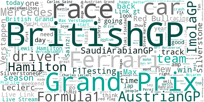
Shape and Mask Images:
The final advanced customization technique we’ll explore is the use of mask images to create word clouds in specific shapes.
- Creating Masked Word Clouds: Word clouds can be customized into various shapes using image masks. For example, you might use a racing car shape for an F1-themed word cloud. Masks allow for creative visualizations that enhance the thematic relevance of your word cloud. When choosing a mask image, it’s essential to select one that is simple and not overly complicated, as well as an image with high contrast against the background. This approach ensures the word cloud remains clear and visually impactful, with the text legible within the mask shape.
- Resizing and Scaling: Proper handling of image sizes and resolutions is crucial to ensure clarity and impact. The dimensions of the word cloud should match those of the mask image to maintain visual integrity.
Here’s an example of how to use a mask image to generate a word cloud:
# Define the path to the mask image
mask_path = 'path/to/your/mask_image.png'  # Update this path to your mask image location

# Load the mask image
mask_image = np.array(Image.open(mask_path))

# Generate the word cloud with the mask and custom settings
wordcloud = WordCloud(
    width=mask_image.shape[1],  # Match the mask image width
    height=mask_image.shape[0],  # Match the mask image height
    background_color='white',  # Light background for contrast
    colormap=f1_theme_cmap,  # Use a predefined colormap object
    stopwords=custom_stopwords,  # Apply custom stopwords
    mask=mask_image  # Apply the mask image
).generate(all_text)

# Display the word cloud
plt.figure(figsize=(11.25, 6.25))  # Adjust figure size for better display
plt.imshow(wordcloud, interpolation='bilinear')  # Smooth rendering
plt.axis('off')  # Hide the axis
plt.title('Enhanced F1 Tweet Word Cloud: Custom Stopwords, Colormap, and Mask Image')  # Add a title
plt.show()  # Render the plot
Visualization and Aesthetics
The customizations we’ve discussed boost your word clouds’ information. However, make sure they are also visually appealing and readable. Here are some tips to enhance your word cloud’s aesthetics.
Improving Readability: Clear text is vital. Adjust font sizes and spacing for better visibility.
Background and Contrast: Choose the right background color. Ensure there’s enough contrast between the text and the background. This makes the words stand out and grabs attention.
Focusing on these visual tweaks can elevate your word clouds. They will offer insights and look professional. Such considerations greatly improve your data analysis projects.
Conclusion
This post covered making better word clouds. First, we explored basic and advanced techniques. We learned to use custom stopwords to remove unwanted words. Then, we added color with both predefined and custom colormaps. Finally, we used mask images for unique shapes. These methods enhance both the information and the look of word clouds.
I hope this guide made word clouds clearer for you. The libraries in Python and R are good starting points. However, they may limit visibility and customization. If word clouds are vital for your project or analysis, consider tools like Word Cloud Plus, Josh Davies, and Word Art.
For more on the Python ‘wordcloud’ library, visit its official PyPI page.
Thank you for reading about improving word clouds. I hope the techniques and insights boost your data analysis and storytelling. The code related to this post is available in my GitHub repository: GitHub Repo Link.